3. Quickstart

Here we provide usage examples of web tools and Python package, as well as the installation method of the latter.

3.1. Web Tools

Note: We will not elaborate on the meanings of each parameter in this chapter’s tutorial. If you want to know about it, please refer to here.

3.1.1. Usage Examples

3.1.1.1. Z-curve Plotter

In this section, we will show how to visualize and compare genomes of different species strains, and find the DNA replication origins of them (for bacteria). First, choose 2 genomes and upload them. For convenience, We upload the example sequences (E. coli SMS-3-5 NC_010498.1 and MG1655 NC_000913.3) through the online download function, which is able to fetch data from NCBI Nucleotide database. You can also upload your own files to complete this step.

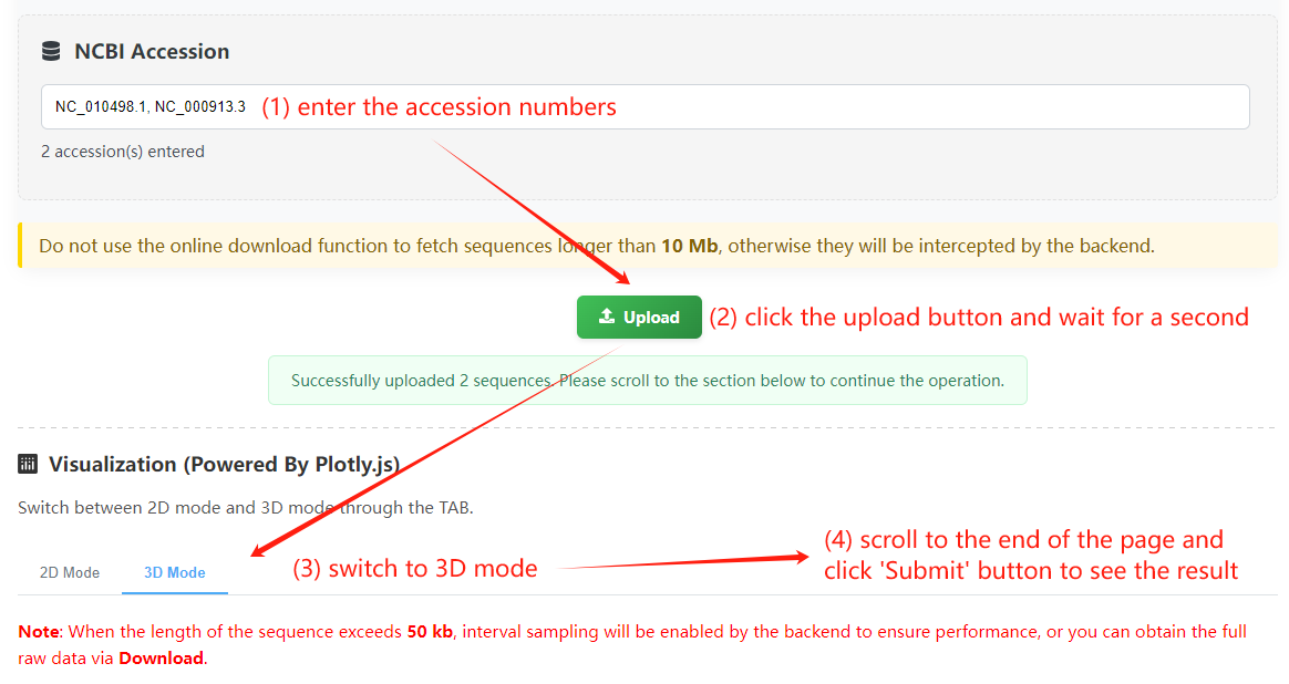
Then switch the plotter mode to 3D mode, adjust the settings and submit via the button below. Our example uses the original version of the Z curve, so we just use the default values. Finally, you can see the 3D representation of the two genomes. Obviously, the two genomes have similar geometric structures, which indicates that they have the same organizational pattern, only differing in local details.

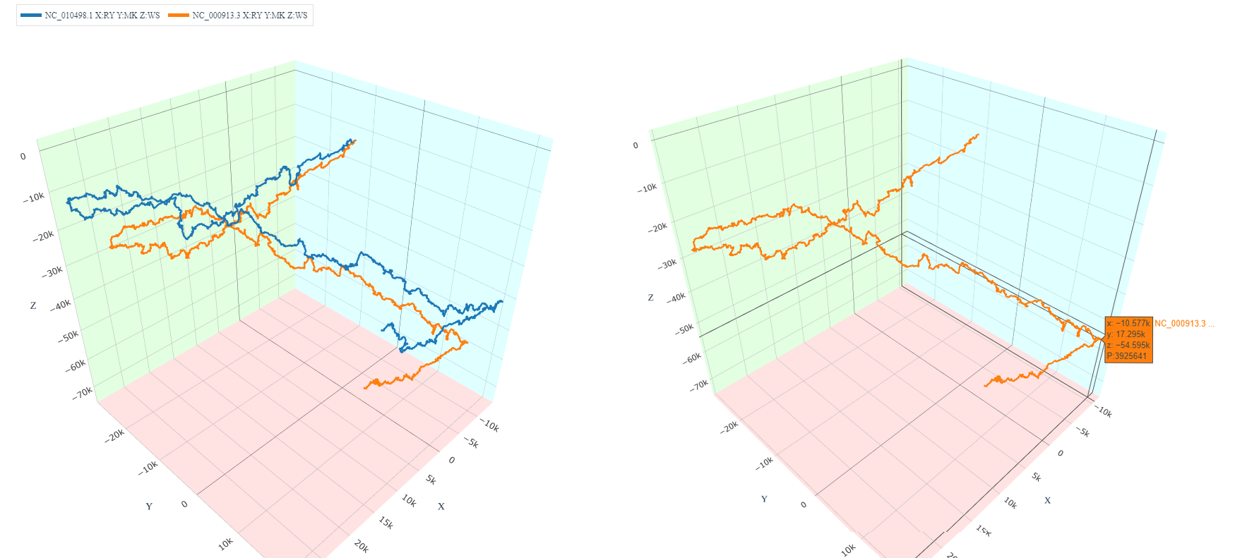
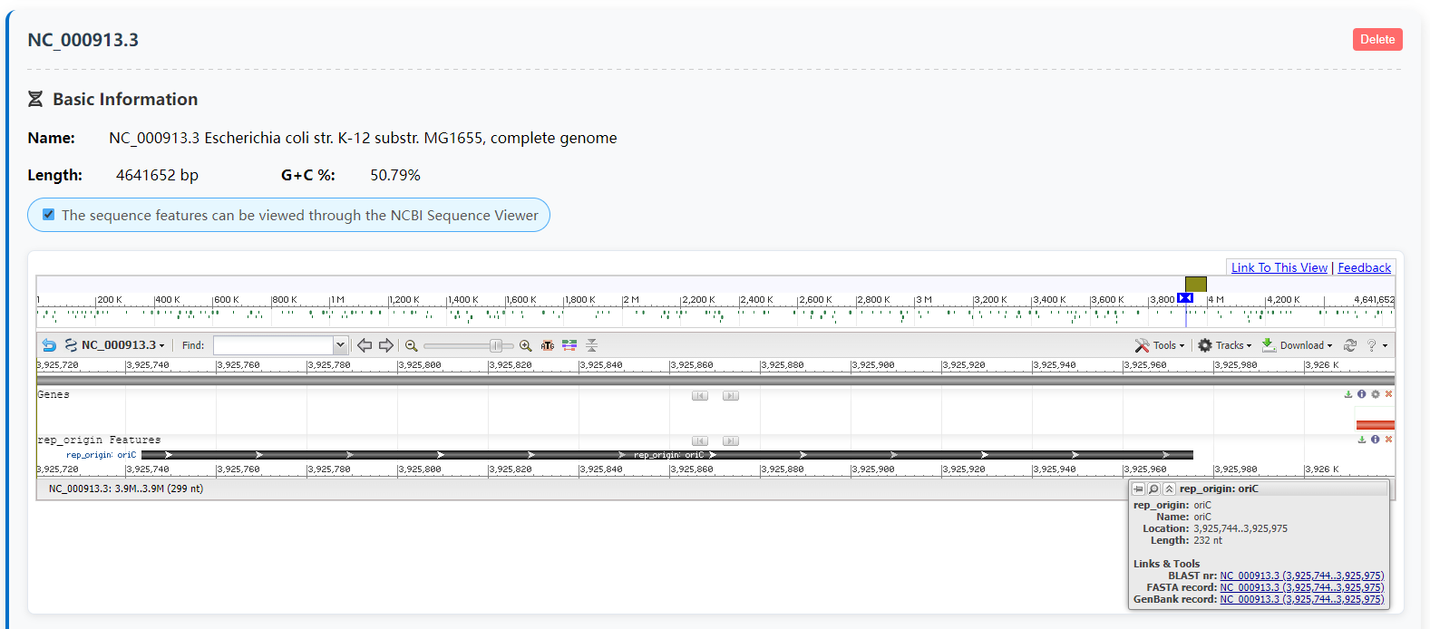
Due to the significant compositional differences between the leading and lagging strands of the bacterial genome, the shape of the Z curve will be in the form of a “Z”, and the replication origin element is located at the turning point. A turning point of SMS-3-5 is 3925461, which corresponds to the replication initiation point (3925744..3925975) as annotated by NCBI.

3.2. Python Package

3.2.1. Installation

Python includes the package management system pip which should allow you to install ZcurvePy and its dependencies if needed, as well as upgrade or uninstall with just one command in the terminal:

python -m pip install zcurvepy
python -m pip install --upgrade zcurvepy

python -m pip uninstall zcurvepy

Starting from 1.5.11, the return value types of some frequently used API functions have been modified from Python list to Numpy ndarray. Therefore, please install Numpy 1.x before compiling and installing.

python -m pip install "numpy>=1.21,<2.0"

3.2.1.1. Python Requirements

Python 3.7, 3.8, 3.9, 3.10, 3.11, 3.12 are supported. We currently recommend using Python 3.9.6 (https://www.python.org/downloads/release/python-396/)

3.2.1.2. Operating System

Windows 10/11, macOS, and Linux running on x86_64 arch are supported. Note that some features of Matplotlib may not work on systems without a graphic interface (e.g., RedHat).

3.2.2. Usage Examples

1. Generate Z-curves and derivatives
   (1) Python API implementation:

   from ZcurvePy import ZcurvePlotter
   from ZcurvePy.Util import download_acc
   from Bio.SeqIO import read
   import matplotlib.pyplot as plt
   # Download genomes (Please wait for several seconds)
   save_paths = download_acc("NC_000854.2,NC_000868.1")
   ax3d = plt.figure().add_subplot(projection='3d')
   ax2d = plt.figure().add_subplot()
   for save_path in save_paths:
       record = read(save_path, "fasta")
       # Calculate components of smoothed Z-curve
       plotter = ZcurvePlotter(record)
       n, x, y, _ = plotter.z_curve(window=1000)
       zp, _ = plotter.z_prime_curve(window=1000, return_n=False)
       # Matplotlib 2D display
       ax2d.plot(n[::10], x[::10], label=f"{record.id} RY-disparity")
       ax2d.plot(n[::10], y[::10], label=f"{record.id} MK-disparity")
       ax2d.plot(n[::10], zp[::10], label=f"{record.id} Z'n curve")
       ax2d.legend()
       # Matplotlib 3D display
       ax3d.plot(x[::10], y[::10], zp[::10], label=f"{record.id} Z-curve")
       ax3d.legend()
   plt.show()
   

   (2) Commandline usage:
   For plotting curves in 2D mode:

   zcurve-plotter -a NC_000854.2,NC_000868.1 -s settings.json -p curves.png -o curves_2d.json
   

   and for plotting curves in 3D mode:

   zcurve-plotter-3d -a NC_000854.2,NC_000868.1 -s settings.json -p curves.png -o curves_3d.json
   

   where the settings should be a JSON like:

   {
       "plotter": [
           {
               "window": 10000, 
               "intv": 100,
               "curve2d": "RY,MK,ZP",
               "curve3d": "RY:MK:ZP"
           },
           {
               "window": 10000, 
               "intv": 100,
               "curve2d": "RY,MK,ZP",
               "curve3d": "RY:MK:ZP"
           }
       ]
   }
   

   Note that the Z-curve Plotter’s 3D mode allows you to select 3 of the 11 curves as components of x,y, and z.
   For more help information about the setting file, please enter:

   zcurve-plotter --help
   

2. Extract Z-curve parameter features
   (1) Python API implementation:

   from ZcurvePy.Util import download_acc, extract_CDS
   import numpy as np
   save_paths = download_acc("NC_000854.2", __name__, "gb")
   records = extract_CDS(save_paths[0])
   
   from ZcurvePy import ZcurveEncoder
   def encoding(record):
       """ simple batch processing """
       encoder = ZcurveEncoder(record)
       # Calculate and concatenate 765-bit Z-curve transform
       feature = encoder.mononucl_phase_transform(freq=True)
       feature = np.concatenate((feature, encoder.dinucl_phase_transform(freq=True)))
       feature = np.concatenate((feature, encoder.trinucl_phase_transform(freq=True)))
       feature = np.concatenate((feature, encoder.k_nucl_phase_transform(k=4, freq=True)))
       return feature
   
   features = np.array([encoding(record) for record in records])
   print(features.shape)
   

   or use another more powerful API to implement multi-threading:

   from ZcurvePy import BatchZcurveEncoder
   # Define the hyper-paramsfor 765-bit Z-curve transform
   hyper_params = [
       {"k": 1, "freq": True}  # Same as mononucl_phase_transform(freq=True)
       {"k": 2, "freq": True}  # Same as dinucl_phase_transform(freq=True)
       {"k": 3, "freq": True}  # Same as trinucl_phase_transform(freq=True)
       {"k": 4, "freq": True}  # Same as k_nucl_phase_transform(k=4, freq=True)
   ]
   encoder = BatchZcurveEncoder(hyper_params, n_jobs=8)
   features = encoder(records)
   

   (2) Commandline usage:

   zcurve-encoder -a NC_000854.2 -s settings.json -e True -o features.csv
   

   where the setting file should be a JSON like:

   {
       "encoder": {
           "hyper_params": [
               {"k": 1, "freq": true},
               {"k": 2, "freq": true},
               {"k": 3, "freq": true},
               {"k": 4, "freq": true}
           ],
           "n_jobs": 8
       }
   }
   

   For more help information about the setting file, please enter:

   zcurve-encoder --help
   

3. Segmentation for DNA sequences Python API implementation:

   from ZcurvePy.Util import download_acc
   from Bio.SeqIO import read
   from ZcurvePy import ZcurveSegmenter, ZcurvePlotter
   import matplotlib.pyplot as plt
   # Download data
   path = download_acc("CP001956.1")
   record = read(path[0], "fasta")
   # Segmentation
   segmenter = ZcurveSegmenter(mode='WS', min_len=50000)
   seg_points = segmenter.run(record)
   # Calculate z' curve for visualization
   plotter = ZcurvePlotter(record)
   n, zp, _ = plotter.z_prime_curve()
   # Visualization
   for point, _ in seg_points:
       plt.axvline(point, color='red')
   plt.plot(n, zp)
   plt.show()
   

   Commandline usage:

   zcurve-segmenter -a CP001956.1 -m WS -l 50000 -o seg_points.csv -s True
   

4. Build a simple gene recognizer
   This is an example of training a gene recognition model for Escherichia coli :

   # We recommend turning on the acceleration system on Intel platforms
   from sklearnex import patch_sklearn
   patch_sklearn()
   from ZcurvePy.Util import download_acc, extract_CDS
   from ZcurvePy import ZcurveBuilder
   from Bio.SeqIO import read, parse
   # Load positive dataset
   path = download_acc("NC_000913.3", __name__, "gb")[0]
   pos_dataset = extract_CDS(path)
   builder = ZcurveBuilder(standard=True, n_jobs=8)
   builder.fit(pos_dataset)
   # Some sample sequences
   records = parse("samples.fa", "fasta")
   results = builder.predict(records)