6. Python API

We listed a table here corresponding to that in the Introduction to better help readers sort out the logical relationship between the various curve-related APIs:

Cumulative Curve	Profile Curve	Segmentation Method	Order Index S(P)*
z_curve	**	genome_dS_curve	genome_order_index
RY_disparity	x_prime_curve	RY_dS_curve	RY_order_index
MK_disparity	y_prime_curve	MK_dS_curve	MK_order_index
WS_disparity	z_prime_curve	WS_dS_curve	WS_order_index
AT_disparity	AT_prime_curve	AT_dS_curve	AT_order_index
GC_disparity	GC_prime_curve	GC_dS_curve	GC_order_index
***	CpG_prime_curve	CpG_dS_curve	CpG_order_index

*     The order index was treated as a feature of the sequence for machine learning in earlier studies, so it is integrated under the ZcurveEncoder. The other APIs are integrated under ZcurvePlotter.
**    Z profile curves in 3D form are generally not used for visualization, but their parameters are used for gene starting point prediction, so we only provide it in “profile” mode of BatchZcurvePlotter to batch the dataset. You can use bulk interfaces (x_prime_curve, y_prime_curve, z_prime_curve) to implement it in 3D form as well.
***  The geometry of the CpG-disparity curve is not obvious, so we do not provide a standard API. Readers may implement and explore its features on their own.

6.1. ZcurvePy

This is the Python package __init__ module of released ZcurvePy package. All the C/C++ apis can be called through this module. If you don’t want to import additional third-party modules (e.g. modules from scikit-learn) or APIs written in pure Python provided by ZcurvePy (e.g. ZcurveBuilder), use import _ZcurvePy instead of import ZcurvePy.

6.1.1. ZcurvePlotter

A simple API for plotting a nucleotide sequence to Z-curve or do segmentation based on order index. Multi-thread is not supported by this API. If you want to plot Z-curve for a large dataset using multi-thread, use BatchZcurvePlotter instead. This API only returns coordinate information and provides no graphical operations. If you want visual curves, use commandline tools or program it by yourself using visualization library like Matplotlib and Plotly.

6.1.1.1. ZcurvePlotter.__init__

__init__ method of _ZcurvePy.ZcurvePlotter
Args:

• seq_or_record:
  Object that stores information of nucleic sequence. str, Bio.Seq.Seq, Bio.SeqRecord.SeqRecord and many other types are supported.

Returns:

• plotter (object):
  _ZcurvePy.ZcurvePlotter

6.1.1.2. ZcurvePlotter.z_curve

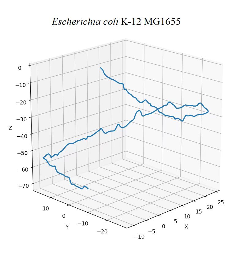
Convert a DNA sequence or RNA sequence to Z-curve.

Background
Z-curve theory is a geometrical approach to genome analysis. The Z-curve is a three-dimensional curve that represents a DNA sequence in the sense that each can be uniquely reconstructed given the other.The Z-curve, therefore, contains all the information that the corresponding DNA sequence carries.

Definition
Let \(A_n\), \(G_n\), \(C_n\) and \(T_n\) be the count of A, G, C and T of a subsequence consisting of the first \(n\) nucleotides of a DNA, s.t.

\(x_n = (A_n + G_n) - (C_n + T_n)\)
\(y_n = (A_n + C_n) - (G_n + T_n), n=1,2,3 ...,N\)
\(z_n = (A_n + T_n) - (G_n + C_n)\)

The \(x_n\), \(y_n\), \(z_n\) can be drawn in a three-dimensional rectangular coordinate system, or take the length of the sequence as the horizontal axis and be drawn in three plane coordinate systems. In this process, both global and local features of the sequence are well visualized.

This curve could be smoothed using mean-smoothing method.

Application Scene
Genome visualization; Replication origins prediction; Machine learning

Usage Example

from Bio import SeqIO
from ZcurvePy import ZcurvePlotter
import matplotlib.pyplot as plt

record = SeqIO.read("e_coli.fa", "fasta")
plotter = ZcurvePlotter(record)
x, y, z = plotter.z_curve(window=10000, return_n=False)
# n, x, y, z = plotter.z_curve(window=10000)

fig = plt.figure(figsize=(10, 10))
ax3d = fig.add_subplot(projection='3d')
ax3d.plot(x, y, z)
ax3d.set_xlabel("X", labelpad=10)
ax3d.set_ylabel("Y", labelpad=10)
ax3d.set_zlabel("Z", labelpad=10)
plt.show()

Args:

• window (int):
  Window size used by mean-smoothing method. If a value <= 0 is given, do nothing and return the original curve data. (Default: 0)

• return_n (bool):
  Return the sequence length axis or not. (Default: True)

Returns:

• n (ndarray):
  The sequence length axis.

• x (ndarray):
  The x values of the Z-curve.

• y (ndarray):
  The y values of the Z-curve.

• z (ndarray):
  The z values of the Z-curve

6.1.1.3. ZcurvePlotter.RY_disparity

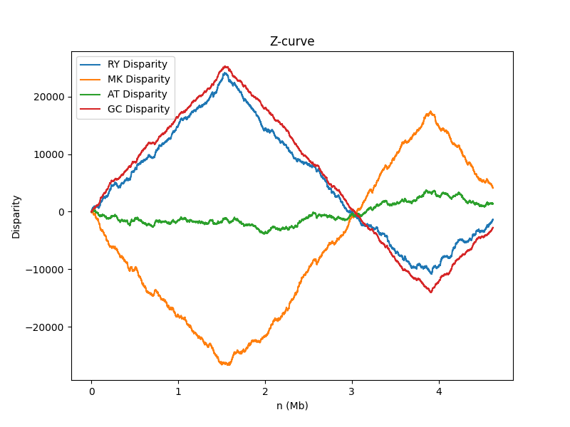
Returns the x values of the Z-curve (RY-disparity).

Definition
Let \(A_n\), \(G_n\), \(C_n\) and \(T_n\) be the count of A, G, C and T of a subsequence consisting of the first \(n\) nucleotides of a DNA, s.t.

\(x_n = (A_n + G_n) - (C_n + T_n), n=1,2,3 ...,N\)

This curve could be smoothed using mean-smoothing method.

Application Scene
Genome visualization; Replication origins prediction; Machine learning

Usage Example

from Bio import SeqIO
from ZcurvePy import ZcurvePlotter
import matplotlib.pyplot as plt

record = SeqIO.read("e_coli.fa", "fasta")
plotter = ZcurvePlotter(record)
n, x = plotter.RY_disparity(window=100)
# x = plotter.RY_disparity(window=100, return_n=False)
plt.plot(n, x)
plt.xlabel('n (bp)', labelpad=10)
plt.ylabel('RY Disparity', labelpad=10)
plt.show()

Args:

• window (int):
  Window size used by mean-smoothing method. If a value <= 0 is given, do nothing and return the original curve data. (Default: 0)

• return_n (bool):
  Return the sequence length axis or not. (Default: True)

Returns:

• n (ndarray):
  The sequence length axis.

• x (ndarray):
  The x values of the Z-curve.

6.1.1.4. ZcurvePlotter.MK_disparity

Returns the y values of the Z-curve (MK-disparity).

Definition
Let \(A_n\), \(G_n\), \(C_n\) and \(T_n\) be the count of A, G, C and T of a subsequence consisting of the first \(n\) nucleotides of a DNA, s.t.

\(y_n = (A_n + C_n) - (G_n + T_n), n=1,2,3 ...,N\)

This curve could be smoothed using mean-smoothing method.

Application Scene
Genome visualization; Replication origins prediction; Machine learning

Usage Example

from Bio import SeqIO
from ZcurvePy import ZcurvePlotter
import matplotlib.pyplot as plt

record = SeqIO.read("e_coli.fa", "fasta")
plotter = ZcurvePlotter(record)
n, y = plotter.MK_disparity(window=100)
# y = plotter.MK_disparity(window=100, return_n=False)
plt.plot(n, y)
plt.xlabel('n (bp)', labelpad=10)
plt.ylabel('MK Disparity', labelpad=10)
plt.show()

For the visual displaying example, please see ZcurvePlotter.RY_disparity
Args:

• window (int):
  Window size used by mean-smoothing method. If a value <= 0 is given, do nothing and return the original curve data. (Default: 0)

• return_n (bool):
  Return the sequence length axis or not. (Default: True)

Returns:

• n (ndarray):
  The sequence length axis.

• y (ndarray):
  The y values axis of the Z-curve.

6.1.1.5. ZcurvePlotter.WS_disparity

Returns the z values of the Z-curve (WS-disparity).

Definition
Let \(A_n\), \(G_n\), \(C_n\) and \(T_n\) be the count of A, G, C and T of a subsequence consisting of the first \(n\) nucleotides of a DNA, s.t.

\(z_n = (A_n + T_n) - (G_n + C_n), n=1,2,3 ...,N\)

This curve could be smoothed using mean-smoothing method.

Application Scene
Genome visualization; Replication origins prediction; Machine learning

Usage Example

from Bio import SeqIO
from ZcurvePy import ZcurvePlotter
import matplotlib.pyplot as plt

record = SeqIO.read("e_coli.fa", "fasta")
plotter = ZcurvePlotter(record)
n, z = plotter.WS_disparity(window=100)
# z = plotter.WS_disparity(window=100, return_n=False)
plt.plot(n, z)
plt.xlabel('n (bp)', labelpad=10)
plt.ylabel('WS Disparity', labelpad=10)
plt.show()

The local geometry of WS-display is not significant in the vast majority of species. (due to stable GC content)
Args:

• window (int):
  Window size used by mean-smoothing method. If a value <= 0 is given, do nothing and return the original curve data. (Default: 0)

• return_n (bool):
  Return the sequence length axis or not. (Default: True)

Returns:

• n (ndarray):
  The sequence length axis.

• z (ndarray):
  The z values axis of the Z-curve.

6.1.1.6. ZcurvePlotter.AT_disparity

Returns AT-disparity.

Definition
Let \(A_n\) and \(T_n\) be the count of A and T of a subsequence consisting of the first \(n\) nucleotides of a DNA, s.t.

\(d_{\rm AT}(n) = A_n - T_n, n=1,2,3 ...,N\)

This curve could be smoothed using mean-smoothing method.

Application Scene
Genome visualization

Usage Example

from Bio import SeqIO
from ZcurvePy import ZcurvePlotter
import matplotlib.pyplot as plt

record = SeqIO.read("e_coli.fa", "fasta")
plotter = ZcurvePlotter(record)
n, d = plotter.AT_disparity(window=100)
# d = plotter.AT_disparity(window=100, return_n=False)
plt.plot(n, d)
plt.xlabel('n (bp)', labelpad=10)
plt.ylabel('AT Disparity', labelpad=10)
plt.show()

For the visual displaying example, please see ZcurvePlotter.RY_disparity
Args:

• window (int):
  Window size used by mean-smoothing method. If a value <= 0 is given, do nothing and return the original curve data. (Default: 0)

• return_n (bool):
  Return the sequence length axis or not. (Default: True)

Returns:

• n (ndarray):
  The sequence length axis.

• d (ndarray):
  The AT-disparity values.

6.1.1.7. ZcurvePlotter.GC_disparity

Returns GC-disparity.

Definition
Let \(G_n\) and \(C_n\) be the count of A and T of a subsequence consisting of the first \(n\) nucleotides of a DNA, s.t.

\(d_{\rm GC}(n) = G_n - C_n, n=1,2,3 ...,N\)

This curve could be smoothed using mean-smoothing method.

Application Scene
Genome visualization

Usage Example

from Bio import SeqIO
from ZcurvePy import ZcurvePlotter
import matplotlib.pyplot as plt

record = SeqIO.read("e_coli.fa", "fasta")
plotter = ZcurvePlotter(record)
n, f = plotter.GC_disparity(window=1000)
# f = plotter.GC_disparity(window=1000, return_n=False)
plt.plot(n, f)
plt.xlabel('n (bp)', labelpad=10)
plt.ylabel('GC Disparity', labelpad=10)
plt.show()

For the visual displaying example, please see ZcurvePlotter.RY_disparity
Args:

• window (int):
  Window size used by mean-smoothing method. If a value <= 0 is given, do nothing and return the original curve data. (Default: 0)

• return_n (bool):
  Return the sequence length axis or not. (Default: True)

Returns:

• n (ndarray):
  The sequence length axis.

• f (ndarray):
  The GC-disparity values.

6.1.1.8. ZcurvePlotter.AT_skew

Returns sliding window calculated AT-skew.

Definition
Let \(A^k_n\) and \(T^k_n\) be the count of A and T of a subsequence consisting of \(k\) nucleotides (window size) at position \(n\) of a DNA, s.t.

\(skew_{\rm AT}(n,k) = (A^k_n - T^k_n) / (A^k_n + T^k_n), n=1,2,3 ...,N\)

Application Scene
Genome visualization

Usage Example

from Bio import SeqIO
from ZcurvePy import ZcurvePlotter
import matplotlib.pyplot as plt

record = SeqIO.read("e_coli.fa", "fasta")
plotter = ZcurvePlotter(record)
n, a = plotter.AT_skew(window=100)
# a = plotter.AT_skew(window=100, return_n=False)
plt.plot(n, a)
plt.xlabel('n (bp)', labelpad=10)
plt.ylabel('AT Skew', labelpad=10)
plt.show()

Args:

• window (int):
  Window size (>= 50) used by sliding window method. (Default: 100)

• return_n (bool):
  Return the sequence length axis or not. (Default: True)

Returns:

• n (ndarray):
  The sequence length axis.

• a (ndarray):
  The AT-skew values.

6.1.1.9. ZcurvePlotter.GC_skew

Returns sliding window calculated GC-skew.

Definition
Let \(G^k_n\) and \(C^k_n\) be the count of G and C of a subsequence consisting of \(k\) nucleotides (window size) at position \(n\) of a DNA, s.t.

\(skew_{\rm GC}(n,k) = (G^k_n - C^k_n) / (G^k_n + C^k_n), n=1,2,3 ...,N\)

Application Scene
Genome visualization

Usage Example

from Bio import SeqIO
from ZcurvePy import ZcurvePlotter
import matplotlib.pyplot as plt

record = SeqIO.read("e_coli.fa", "fasta")
plotter = ZcurvePlotter(record)
n, g = plotter.GC_skew(window=1000)
# g = plotter.GC_skew(window=1000, return_n=False)
plt.plot(n, g)
plt.xlabel('n (bp)', labelpad=10)
plt.ylabel('GC Skew', labelpad=10)
plt.show()

Args:

• window (int):
  Window size (>= 50) used by sliding window method. (Default: 100)

• return_n (bool):
  Return the sequence length axis or not. (Default: True)

Returns:

• n (ndarray):
  The sequence length axis.

• g (ndarray):
  The GC-skew values.

6.1.1.10. ZcurvePlotter.AT_fraction

Returns sliding window calculated AT fraction.

Definition
Let \(A^k_n\), \(T^k_n\), \(G^k_n\) and \(C^k_n\) be the count of G and C of a subsequence consisting of \(k\) nucleotides (window size) at position \(n\) of a DNA, s.t.

\(fraction_{AT}(n, k) = (A^k_n + T^k_n) / (A^k_n + T^k_n + G^k_n + C^k_n), n=1,2,3 ...,N\)

Application Scene
Genome visualization

Usage Example

from Bio import SeqIO
from ZcurvePy import ZcurvePlotter
import matplotlib.pyplot as plt

record = SeqIO.read("e_coli.fa", "fasta")
plotter = ZcurvePlotter(record)
n, g = plotter.AT_fraction(window=1000)
# g = plotter.AT_fraction(window=1000, return_n=False)
plt.plot(n, g)
plt.xlabel('n (bp)', labelpad=10)
plt.ylabel('AT Fraction', labelpad=10)
plt.show()

6.1.1.11. ZcurvePlotter.GC_fraction

Returns sliding window calculated GC fraction.

Definition
Let \(A^k_n\), \(T^k_n\), \(G^k_n\) and \(C^k_n\) be the count of G and C of a subsequence consisting of \(k\) nucleotides (window size) at position \(n\) of a DNA, s.t.

\(fraction_{GC}(n, k) = (G^k_n + C^k_n) / (A^k_n + T^k_n + G^k_n + C^k_n), n=1,2,3 ...,N\)

Application Scene
Genome visualization

Usage Example

from Bio import SeqIO
from ZcurvePy import ZcurvePlotter
import matplotlib.pyplot as plt

record = SeqIO.read("e_coli.fa", "fasta")
plotter = ZcurvePlotter(record)
n, g = plotter.GC_fraction(window=1000)
# g = plotter.GC_fraction(window=1000, return_n=False)
plt.plot(n, g)
plt.xlabel('n (bp)', labelpad=10)
plt.ylabel('GC Fraction', labelpad=10)
plt.show()

6.1.1.12. ZcurvePlotter.x_prime_curve

Calculate x’ values and the slope ‘k’.

Background
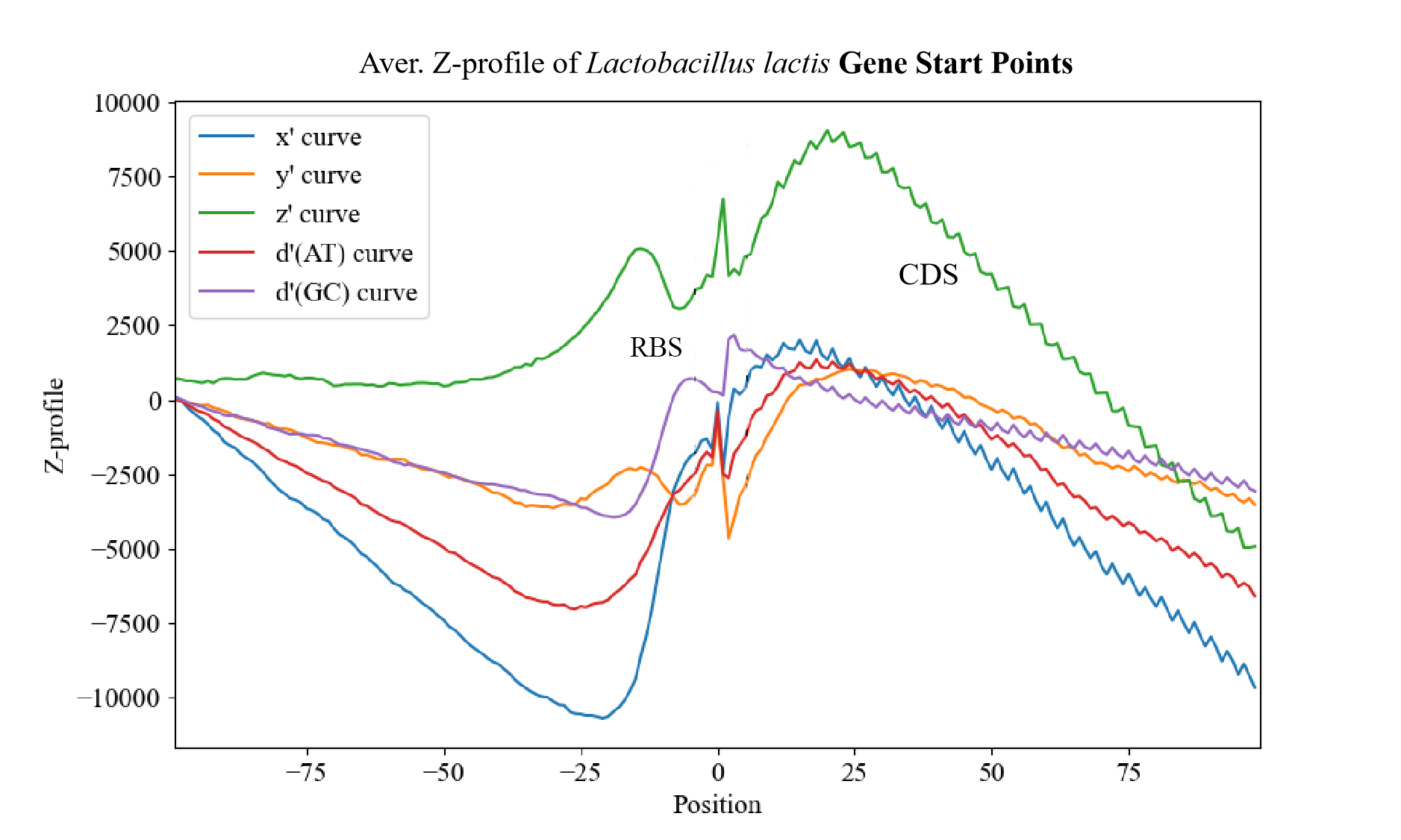
The different patterns of the species-specific, conserved nucleotide distribution are helpful to extract some recognition variables to identify gene starts. In prokaryotic genomes, a major jump in xn occurs in the region of −14 to −7 for the true start codons, but not for the non-coding ORFs. It is likely caused by purine-rich SD sequence.Therefore the features of mononucleotide frequencies near the true start codons are notably different from those of the upstream and downstream false starts.

Definition
Let \(A_n\), \(G_n\), \(C_n\) and \(T_n\) be the count of A, G, C and T of a subsequence consisting of the first \(n\) nucleotides of a DNA, s.t.

\(x_n = (A_n + G_n) - (C_n + T_n), n=1,2,3 ...,N\)

apply a linear fit to the curve based on least square method, then a slope ‘k’ is obtained, s.t.

\(x'_n = x_n - kn, n=1,2,3 ...,N\)

Application Scene
Genome visualization; Gene start sites prediction

Usage Example

from Bio import SeqIO
from ZcurvePy import ZcurvePlotter
import matplotlib.pyplot as plt

record = SeqIO.read("e_coli.fa", "fasta")
plotter = ZcurvePlotter(record)
n, xp, k = plotter.x_prime_curve(window=100)
# xp, k = plotter.x_prime_curve(window=100, return_n=False)
plt.plot(n, xp)
plt.xlabel('n (bp)', labelpad=10)
plt.ylabel("x'", labelpad=10)
plt.show()

Args:

• window (int):
  Window size used by mean-smoothing method. If a value <= 0 is given, do nothing and return the original curve data. (Default: 0)

• return_n (bool):
  return the sequence length axis or not. (Default: True)

Returns:

• n (ndarray):
  The sequence length axis.

• xp (ndarray):
  The x’ values.

• k (ndarray):
  The slope value ‘k’.

6.1.1.13. ZcurvePlotter.y_prime_curve

Calculate y’ values and the slope ‘k’.

Definition
Let \(A_n\), \(G_n\), \(C_n\) and \(T_n\) be the count of A, G, C and T of a subsequence consisting of the first \(n\) nucleotides of a DNA, s.t.

\(y_n = (A_n + C_n) - (G_n + T_n), n=1,2,3 ...,N\)

apply a linear fit to the curve based on least square method, then a slope ‘k’ is obtained, s.t.

\(y'_n = y_n - kn, n=1,2,3 ...,N\)

Application Scene
Genome visualization; Gene start sites prediction

Usage Example

from Bio import SeqIO
from ZcurvePy import ZcurvePlotter
import matplotlib.pyplot as plt

record = SeqIO.read("e_coli.fa", "fasta")
plotter = ZcurvePlotter(record)
n, yp, k = plotter.y_prime_curve(window=100)
# yp, k = plotter.y_prime_curve(window=100, return_n=False)
plt.plot(n, yp)
plt.xlabel('n (bp)', labelpad=10)
plt.ylabel("y'", labelpad=10)
plt.show()

For the visual displaying example, please see ZcurvePlotter.x_prime_curve

Args:

• window (int):
  Window size used by mean-smoothing method. If a value <= 0 is given, do nothing and return the original curve data. (Default: 0)

• return_n (bool):
  return the sequence length axis or not. (Default: True)

Returns:

• n (ndarray):
  The sequence length axis.

• yp (ndarray):
  The y’ values.

• k (float):
  The slope value ‘k’.

6.1.1.14. ZcurvePlotter.z_prime_curve

Calculate z’ values and the slope ‘k’.

Background
The GC profile is a windowless technique to calculate the G+C content of genomic DNA sequences as well as visualize isolate structures, which is rich of G+C. By this method, the G content can be calculated at different ‘resolution’.In an extreme case, the G content may be computed at a specific point, rather than in a window of finite size. This is particularly useful to analyze the fine variation of base composition along genomic sequences.

Definition
Let \(A_n\), \(G_n\), \(C_n\) and \(T_n\) be the count of A, G, C and T of a subsequence consisting of the first \(n\) nucleotides of a DNA, s.t.

\(z_n = (A_n + T_n) - (G_n + C_n), n=1,2,3 ...,N\)

apply a linear fit to the curve based on least square method, then a slope ‘k’ is obtained, s.t.

\(z'_n = z_n - kn, n=1,2,3 ...,N\)

Application Scene
Genome visualization; Gene start sites prediction

Usage Example

from Bio import SeqIO
from ZcurvePy import ZcurvePlotter
import matplotlib.pyplot as plt

record = SeqIO.read("e_coli.fa", "fasta")
plotter = ZcurvePlotter(record)
n, zp, k = plotter.z_prime_curve(window=100)
# zp, k = plotter.z_prime_curve(window=100, return_n=False)
plt.plot(n, zp)
plt.xlabel('n (bp)', labelpad=10)
plt.ylabel("z'", labelpad=10)
plt.show()

Args:

• window (int):
  Window size used by mean-smoothing method. If a value <= 0 is given, do nothing and return the original curve data. (Default: 0)

• return_n (bool):
  return the sequence length axis or not. (Default: True)

Returns:

• n (ndarray):
  The sequence length axis.

• zp (ndarray):
  The z’ values.

• k (float):
  The slope value ‘k’.

6.1.1.15. ZcurvePlotter.AT_prime_curve

Calculate d’AT values for AT-disparity.

Definition
Let \(A_n\) and \(T_n\) be the count of A and T of a subsequence consisting of the first \(n\) nucleotides of a DNA, s.t.

\(d_{\rm AT}(n) = A_n - T_n, n=1,2,3 ...,N\)

apply a linear fit to the curve based on least square method, then a slope ‘k’ is obtained, s.t.

\(d'_{\rm AT}(n) = d_{\rm AT}(n) - kn, n=1,2,3 ...,N\)

Application Scene
Genome visualization

Usage Example

from Bio import SeqIO
from ZcurvePy import ZcurvePlotter
import matplotlib.pyplot as plt

record = SeqIO.read("e_coli.fa", "fasta")
plotter = ZcurvePlotter(record)
n, dp, k = plotter.AT_prime_curve(window=100)
# dp, k = plotter.AT_prime_curve(window=100, return_n=False)
plt.plot(n, dp)
plt.xlabel('n (bp)', labelpad=10)
plt.ylabel("d'AT", labelpad=10)
plt.show()

For the visual displaying example, please see ZcurvePlotter.x_prime_curve

Args:

• window (int):
  Window size used by mean-smoothing method. If a value <= 0 is given, do nothing and return the original curve data. (Default: 0)

• return_n (bool):
  return the sequence length axis or not. (Default: True)

Returns:

• n (ndarray):
  The sequence length axis.

• dp (ndarray):
  The d’AT values.

• k (float):
  The slope value ‘k’.

6.1.1.16. ZcurvePlotter.GC_prime_curve

Calculate d’GC values for GC-disparity.

Definition
Let \(G_n\) and \(C_n\) be the count of G and C of a subsequence consisting of the first \(n\) nucleotides of a DNA, s.t.

\(d_{\rm GC}(n) = G_n - C_n, n=1,2,3 ...,N\)

apply a linear fit to the curve based on least square method, then a slope ‘k’ is obtained, s.t.

\(d'_{\rm GC}(n) = d_{\rm GC}(n) - kn, n=1,2,3 ...,N\)

Application Scene
Genome visualization

Usage Example

from Bio import SeqIO
from ZcurvePy import ZcurvePlotter
import matplotlib.pyplot as plt

record = SeqIO.read("e_coli.fa", "fasta")
plotter = ZcurvePlotter(record)
n, fp, k = plotter.GC_prime_curve(window=100)
# fp, k = plotter.GC_prime_curve(window=100, return_n=False)
plt.plot(n, fp)
plt.xlabel('n (bp)', labelpad=10)
plt.ylabel("d'GC", labelpad=10)
plt.show()

For the visual displaying example, please see ZcurvePlotter.x_prime_curve

Args:

• window (int):
  Window size used by mean-smoothing method. If a value <= 0 is given, do nothing and return the original curve data. (Default: 0)

• return_n (bool):
  return the sequence length axis or not. (Default: True)

Returns:

• n (ndarray):
  The sequence length axis.

• fp (ndarray):
  The d’GC values.

• k (float):
  The slope value ‘k’.

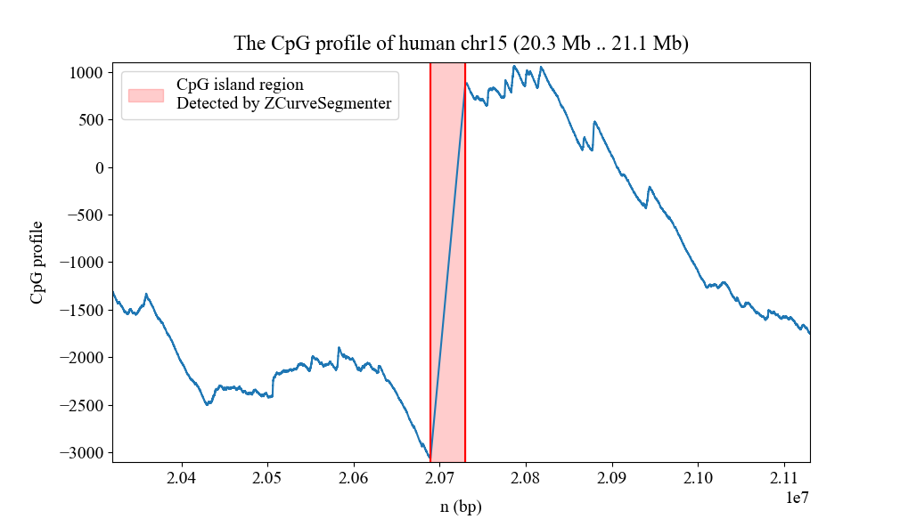
6.1.1.17. ZcurvePlotter.CpG_prime_curve

Calculate z’ values for CpG-profile.

Definition
Let \(CpG_n\) be the count of CpG dinucleotide units in a DNA sequence, s.t.

\(z_n = 2CpG_n - n, n=1,2,3 ...,N\)

apply a linear fit to the curve based on least square method, then a slope ‘k’ is obtained, s.t.

\(z'_n = z_n - kn, n=1,2,3 ...,N\)

Application Scene
Genome visualization

Usage Example

from Bio import SeqIO
from ZcurvePy import ZcurvePlotter
import matplotlib.pyplot as plt

record = SeqIO.read("e_coli.fa", "fasta")
plotter = ZcurvePlotter(record)
n, zp, k = plotter.CpG_prime_curve(window=100)
# zp, k = plotter.CpG_prime_curve(window=100, return_n=False)
plt.plot(n, zp)
plt.xlabel('n (bp)', labelpad=10)
plt.ylabel("CpG-profile", labelpad=10)
plt.show()

For the visual displaying example, please see ZcurvePlotter.z_prime_curve
Args:

• window (int):
  Window size used by mean-smoothing method. If a value <= 0 is given, do nothing and return the original curve data. (Default: 0)

• return_n (bool):
  return the sequence length axis or not. (Default: True)

Returns:

• n (ndarray):
  The sequence length axis.

• zp (ndarray):
  The CpG-profile values.

• k (float):
  The slope value ‘k’.

6.1.1.18. ZcurvePlotter.genome_dS_curve

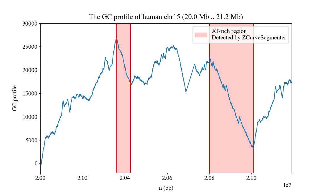
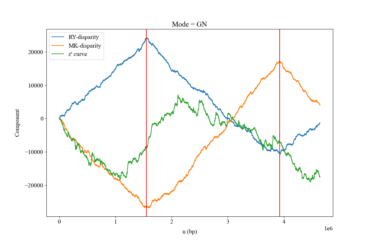
Return dS(P) curve and its max point and max value. Segmentation algorithm for DNA sequences.

Background
Based on the quadratic divergence,the segmentation algorithm to partition a given genome or DNA sequence into compositionally distinct domains is put forward. The algorithm has been applied to segment human chromosome sequences, and the boundaries of isochores for each chromosome were obtained. Compared with the results obtained by using the entropic segmentation algorithm based on the Jensen-Shannon divergence, both algorithms resulted in all identical coordinates of segmentation points. An explanation of the equivalence of the two segmentation algorithms is presented. The new algorithm has a number of advantages. Particularly, it is much simpler and faster than the entropy-based method. Therefore, the new algorithm is more suitable for analyzing long genome sequences, such as human and other newly sequenced eukaryotic genome sequences.

Definition
Let \(a_n\), \(g_n\), \(c_n\) and \(t_n\) be the frequency of A, G, C, T of a subsequence consisting of the first \(n\) nucleotides of a DNA, such that

\(S_n({\rm P}) = a_n^2 + t_n^2 + c_n^2 + g_n^2, n=1,2,3...,N\)

and denote that of the rest of the sequence by \(S({\rm Q})\), such that we have

\(dS_n({\rm P}) = w_1S_n({\rm P}) + w_2S_n({\rm Q}) - S(w_1{\rm P} + w_2{\rm Q}), n=1,2,3...,N\)

the max point of the \(dS_n({\rm P})\) is the segment point in a round of the recursive algorithm.

\(n_{\rm seg} = {\rm argmax}\{dS_n({\rm P})\}\)

Application Scene
Genome segmentation

Usage Example

from Bio import SeqIO
from ZcurvePy import ZcurvePlotter
import matplotlib.pyplot as plt

record = SeqIO.read("e_coli.fa", "fasta")
plotter = ZcurvePlotter(record)
n, sp, mp, mv = plotter.genome_dS_curve(window=10)
# sp, mp, mv = plotter.genome_dS_curve(return_n=False)
# mp, mv = plotter.genome_dS_curve(only_m=True)
plt.plot(n, sp)
plt.axvline(n, mp)
plt.xlabel('n (bp)', labelpad=10)
plt.ylabel("dS(P)", labelpad=10)
plt.show()

Args:

• window (int):
  Window size used by mean-smoothing method. If a value <= 0 is given, do nothing and return the original curve data. (Default: 0)

• return_n (bool):
  return the sequence length axis or not. (Default: True)

• only_m (bool):
  only return max point and max value.

Returns:

• n (ndarray):
  The sequence length axis.

• sp (ndarray):
  The S(P) values axis.

• mp (float):
  The max point of S(P).

• mv (float):
  The max value of S(P).

6.1.1.19. ZcurvePlotter.RY_dS_curve

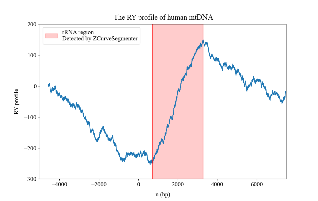
Return dS(P) curve for RY disparity and its max point and max value. Segmentation algorithm for DNA sequences.

Definition
Let \(a_n\), \(g_n\), \(c_n\) and \(t_n\) be the frequency of A, G, C, T of a subsequence consisting of the first \(n\) nucleotides of a DNA, such that

\(S_n({\rm P}) = (a_n + g_n)^2 + (c_n + t_n)^2, n=1,2,3...,N\)

and denote that of the rest of the sequence by \(S({\rm Q})\), such that we have

\(dS_n({\rm P}) = w_1S_n({\rm P}) + w_2S_n({\rm Q}) - S(w_1{\rm P} + w_2{\rm Q}), n=1,2,3...,N\)

the max point of the \(dS_n({\rm P})\) is the segment point in a round of the recursive algorithm.

\(n_{\rm seg} = {\rm argmax}\{dS_n({\rm P})\}\)

Application Scene
Genome segmentation

Usage Example

from Bio import SeqIO
from ZcurvePy import ZcurvePlotter
import matplotlib.pyplot as plt

record = SeqIO.read("e_coli.fa", "fasta")
plotter = ZcurvePlotter(record)
n, sp, mp, mv = plotter.RY_dS_curve(window=10)
# sp, mp, mv = plotter.RY_dS_curve(return_n=False)
# mp, mv = plotter.RY_dS_curve(only_m=True)
plt.plot(n, sp)
plt.axvline(n, mp)
plt.xlabel('n (bp)', labelpad=10)
plt.ylabel("dS(P)", labelpad=10)
plt.show()

Args:

• window (int):
  Window size used by mean-smoothing method. If a value <= 0 is given, do nothing and return the original curve data. (Default: 0)

• return_n (bool):
  return the sequence length axis or not. (Default: True)

• only_m (bool):
  only return max point and max value.

Returns:

• n (ndarray):
  The sequence length axis.

• sp (ndarray):
  The S(P) values axis.

• mp (float):
  The max point of S(P).

• mv (float):
  The max value of S(P).

6.1.1.20. ZcurvePlotter.MK_dS_curve

Return dS(P) curve for MK disparity and its max point and max value. Segmentation algorithm for DNA sequences.

Definition
Let \(a_n\), \(g_n\), \(c_n\) and \(t_n\) be the frequency of A, G, C, T of a subsequence consisting of the first \(n\) nucleotides of a DNA, such that

\(S_n({\rm P}) = (a_n + c_n)^2 + (g_n + t_n)^2, n=1,2,3...,N\)

and denote that of the rest of the sequence by \(S({\rm Q})\), such that we have

\(dS_n({\rm P}) = w_1S_n({\rm P}) + w_2S_n({\rm Q}) - S(w_1{\rm P} + w_2{\rm Q}), n=1,2,3...,N\)

the max point of the \(dS_n({\rm P})\) is the segment point in a round of the recursive algorithm.

\(n_{\rm seg} = {\rm argmax}\{dS_n({\rm P})\}\)

Application Scene
Genome segmentation

Usage Example

from Bio import SeqIO
from ZcurvePy import ZcurvePlotter
import matplotlib.pyplot as plt

record = SeqIO.read("e_coli.fa", "fasta")
plotter = ZcurvePlotter(record)
n, sp, mp, mv = plotter.MK_dS_curve(window=10)
# sp, mp, mv = plotter.MK_dS_curve(return_n=False)
# mp, mv = plotter.MK_dS_curve(only_m=True)
plt.plot(n, sp)
plt.axvline(n, mp)
plt.xlabel('n (bp)', labelpad=10)
plt.ylabel("dS(P)", labelpad=10)
plt.show()

The segmented pattern of bacteria MK disparity is the same as Z-curve, see ZcurvePlotter.genome_order_index
Args:

• window (int):
  Window size used by mean-smoothing method. If a value <= 0 is given, do nothing and return the original curve data. (Default: 0)

• return_n (bool):
  return the sequence length axis or not. (Default: True)

• only_m (bool):
  only return max point and max value.

Returns:

• n (ndarray):
  The sequence length axis.

• sp (ndarray):
  The S(P) values axis.

• mp (float):
  The max point of S(P).

• mv (float):
  The max value of S(P).

6.1.1.21. ZcurvePlotter.WS_dS_curve

Return dS(P) curve for WS disparity and its max point and max value. Segmentation algorithm for DNA sequences.

Definition
Let \(a_n\), \(g_n\), \(c_n\) and \(t_n\) be the frequency of A, G, C, T of a subsequence consisting of the first \(n\) nucleotides of a DNA, such that

\(S_n({\rm P}) = (a_n + t_n)^2 + (c_n + g_n)^2, n=1,2,3...,N\)

and denote that of the rest of the sequence by \(S({\rm Q})\), such that we have

\(dS_n({\rm P}) = w_1S_n({\rm P}) + w_2S_n({\rm Q}) - S(w_1{\rm P} + w_2{\rm Q}), n=1,2,3...,N\)

the max point of the \(dS_n({\rm P})\) is the segment point in a round of the recursive algorithm.

\(n_{\rm seg} = {\rm argmax}\{dS_n({\rm P})\}\)

Application Scene
Genome segmentation

Usage Example

from Bio import SeqIO
from ZcurvePy import ZcurvePlotter
import matplotlib.pyplot as plt

record = SeqIO.read("e_coli.fa", "fasta")
plotter = ZcurvePlotter(record)
n, sp, mp, mv = plotter.WS_dS_curve(window=10)
# sp, mp, mv = plotter.WS_dS_curve(return_n=False)
# mp, mv = plotter.WS_dS_curve(only_m=True)
plt.plot(n, sp)
plt.axvline(n, mp)
plt.xlabel('n (bp)', labelpad=10)
plt.ylabel("dS(P)", labelpad=10)
plt.show()

Args:

• window (int):
  Window size used by mean-smoothing method. If a value <= 0 is given, do nothing and return the original curve data. (Default: 0)

• return_n (bool):
  return the sequence length axis or not. (Default: True)

• only_m (bool):
  only return max point and max value.

Returns:

• n (ndarray):
  The sequence length axis.

• sp (ndarray):
  The S(P) values axis.

• mp (float):
  The max point of S(P).

• mv (float):
  The max value of S(P).

6.1.1.22. ZcurvePlotter.AT_dS_curve

Return dS(P) curve for AT disparity and its max point and max value. Segmentation algorithm for DNA sequences.

Definition
Let \(a_n\), \(g_n\), \(c_n\) and \(t_n\) be the frequency of A, G, C, T of a subsequence consisting of the first \(n\) nucleotides of a DNA, such that

\(S_n({\rm P}) = a_n^2 + t_n^2, n=1,2,3...,N\)

and denote that of the rest of the sequence by \(S({\rm Q})\), such that we have

\(dS_n({\rm P}) = w_1S_n({\rm P}) + w_2S_n({\rm Q}) - S(w_1{\rm P} + w_2{\rm Q}), n=1,2,3...,N\)

the max point of the \(dS_n({\rm P})\) is the segment point in a round of the recursive algorithm.

\(n_{\rm seg} = {\rm argmax}\{dS_n({\rm P})\}\)

Application Scene
Genome segmentation

Usage Example

from Bio import SeqIO
from ZcurvePy import ZcurvePlotter
import matplotlib.pyplot as plt

record = SeqIO.read("e_coli.fa", "fasta")
plotter = ZcurvePlotter(record)
n, sp, mp, mv = plotter.AT_dS_curve(window=10)
# sp, mp, mv = plotter.AT_dS_curve(return_n=False)
# mp, mv = plotter.AT_dS_curve(only_m=True)
plt.plot(n, sp)
plt.axvline(n, mp)
plt.xlabel('n (bp)', labelpad=10)
plt.ylabel("dS(P)", labelpad=10)
plt.show()

The geometric characteristics of the curves AT disparity are not significant.
Args:

• window (int):
  Window size used by mean-smoothing method. If a value <= 0 is given, do nothing and return the original curve data. (Default: 0)

• return_n (bool):
  return the sequence length axis or not. (Default: True)

• only_m (bool):
  only return max point and max value.

Returns:

• n (ndarray):
  The sequence length axis.

• sp (ndarray):
  The S(P) values axis.

• mp (float):
  The max point of S(P).

• mv (float):
  The max value of S(P).

6.1.1.23. ZcurvePlotter.GC_dS_curve

Return dS(P) curve for GC disparity and its max point and max value. Segmentation algorithm for DNA sequences.

Definition
Let \(a_n\), \(g_n\), \(c_n\) and \(t_n\) be the frequency of A, G, C, T of a subsequence consisting of the first \(n\) nucleotides of a DNA, such that

\(S_n({\rm P}) = g_n^2 + c_n^2, n=1,2,3...,N\)

and denote that of the rest of the sequence by \(S({\rm Q})\), such that we have

\(dS_n({\rm P}) = w_1S_n({\rm P}) + w_2S_n({\rm Q}) - S(w_1{\rm P} + w_2{\rm Q}), n=1,2,3...,N\)

the max point of the \(dS_n({\rm P})\) is the segment point in a round of the recursive algorithm.

\(n_{\rm seg} = {\rm argmax}\{dS_n({\rm P})\}\)

Application Scene
Genome segmentation

Usage Example

from Bio import SeqIO
from ZcurvePy import ZcurvePlotter
import matplotlib.pyplot as plt

record = SeqIO.read("e_coli.fa", "fasta")
plotter = ZcurvePlotter(record)
n, sp, mp, mv = plotter.GC_dS_curve(window=10)
# sp, mp, mv = plotter.GC_dS_curve(return_n=False)
# mp, mv = plotter.GC_dS_curve(only_m=True)
plt.plot(n, sp)
plt.axvline(n, mp)
plt.xlabel('n (bp)', labelpad=10)
plt.ylabel("dS(P)", labelpad=10)
plt.show()

The segmented pattern of bacteria GC disparity is the same as RY disparity, see ZcurvePlotter.RY_dS_curve
Args:

• window (int):
  Window size used by mean-smoothing method. If a value <= 0 is given, do nothing and return the original curve data. (Default: 0)

• return_n (bool):
  return the sequence length axis or not. (Default: True)

• only_m (bool):
  only return max point and max value.

Returns:

• n (ndarray):
  The sequence length axis.

• sp (ndarray):
  The S(P) values axis.

• mp (float):
  The max point of S(P).

• mv (float):
  The max value of S(P).

6.1.1.24. ZcurvePlotter.CpG_dS_curve

Return dS(P) curve for CpG-profile and its max point and max value. Segmentation algorithm for DNA sequences.

Definition
Let \(p_n({\rm CpG})\) be the frequency of CpG dinucleotide units in a DNA sequence, such that the CpG order index could be defined as:

\(S_n({\rm P}) = [p_n({\rm CpG})]^2 + [1 - p_n({\rm CpG})]^2, n=1,2,3...,N\)

and denote that of the rest of the sequence by \(S({\rm Q})\), such that we have

\(dS_n({\rm P}) = w_1S_n({\rm P}) + w_2S_n({\rm Q}) - S(w_1{\rm P} + w_2{\rm Q}), n=1,2,3...,N\)

the max point of the \(dS_n({\rm P})\) is the segment point in a round of the recursive algorithm.

\(n_{\rm seg} = {\rm argmax}\{dS_n({\rm P})\}\)

Application Scene
Genome segmentation

Usage Example

from Bio import SeqIO
from ZcurvePy import ZcurvePlotter
import matplotlib.pyplot as plt

record = SeqIO.read("e_coli.fa", "fasta")
plotter = ZcurvePlotter(record)
n, sp, mp, mv = plotter.CpG_dS_curve(window=10)
# sp, mp, mv = plotter.CpG_dS_curve(return_n=False)
# mp, mv = plotter.CpG_dS_curve(only_m=True)
plt.plot(n, sp)
plt.axvline(n, mp)
plt.xlabel('n (bp)', labelpad=10)
plt.ylabel("dS(P)", labelpad=10)
plt.show()

For visual presentation of segmented points, see ZcurvePlotter.CpG_prime_curve
Args:

• window (int):
  Window size used by mean-smoothing method. If a value <= 0 is given, do nothing and return the original curve data. (Default: 0)

• return_n (bool):
  return the sequence length axis or not. (Default: True)

• only_m (bool):
  only return max point and max value.

Returns:

• n (ndarray):
  The sequence length axis.

• sp (ndarray):
  The S(P) values axis.

• mp (float):
  The max point of S(P).

• mv (float):
  The max value of S(P).

6.1.2. ZcurveEncoder

A simple API for converting a DNA sequence to Z-curve parameters, generally used in teaching or learning settings. Multi-thread is not supported by this API. If you want to use multi-thread, please use ZcurvePy.BatchZcurveCoder instead.

6.1.2.1. ZcurveEncoder.__init__

__init__ module of ZcurvePy.ZcurveEncoder

Args:

• seq_or_record:
  object that stores information of nucleic sequence. str, Bio.Seq, Bio.SeqRecord and many other types are supported.

Returns:

• object:
  _ZcurvePy.ZcurveEncoder

6.1.2.2. ZcurveEncoder.mononucl_transform

Do non-phase mononucleotide transformation on a DNA sequence. Generate 3 parameters.

Definition
Let \(A_n\), \(G_n\), \(C_n\), \(T_n\) be the counts of A, G, C, T in a DNA sequence of length \(n\), such that the mononucleotide Z-curve transformation can be:

\(X_n = (A_n + G_n) - (C_n + T_n)\)
\(Y_n = (A_n + C_n) - (G_n + T_n)\)
\(Z_n = (A_n + T_n) - (C_n + G_n)\)

It could also be defined using frequency of bases, which means a kind of normalized version, like:

\(x = [(A_n + G_n) - (C_n + T_n)] / n\)
\(y = [(A_n + C_n) - (G_n + T_n)] / n\)
\(z = [(A_n + T_n) - (C_n + G_n)] / n\)

For more information, please see: ZcurvePy.ZcurveEncoder.k_nucl_phase_transform

Usage Example

from Bio import SeqIO
record = SeqIO.read("example.fa", "fasta")
encoder = ZcurveEncoder(record)
params = encoder.mononucl_transform()
# params = encoder.mononucl_transform(freq=True)

Application Scene
Gene recognition; Machine learning; Deep learning

Args:

• freq (bool):
  do frequencization or not (default: False)

• local (bool):
  use local mode to do frequencization

Returns:

• ndarray:
  Z-curve parameters

6.1.2.3. ZcurveEncoder.dinucl_transform

Do non-phase dinucleotide transformation on a DNA sequence. Generate 12 parameters.

Definition
Let \(NA_n\), \(NG_n\), \(NC_n\), \(NT_n\) be the counts of dinucleotides in a DNA sequence of length \(n\), such that the dinucleotide Z-curve transformation can be:

\(X^{\rm N}_n = (NA_n + NG_n) - (NC_n + NT_n)\)
\(Y^{\rm N}_n = (NA_n + NC_n) - (NG_n + NT_n)\)
\(Z^{\rm N}_n = (NA_n + NT_n) - (NC_n + NG_n)\)

It could also be defined using frequency of bases, which means a kind of normalized version, like:

\(x^{\rm N}_n = [p_n({\rm NA}) + p_n({\rm NG})] - [p_n({\rm NC}) + p_n({\rm NT})]\)
\(y^{\rm N}_n = [p_n({\rm NA}) + p_n({\rm NC})] - [p_n({\rm NG}) + p_n({\rm NT})]\)
\(z^{\rm N}_n = [p_n({\rm NA}) + p_n({\rm NT})] - [p_n({\rm NC}) + p_n({\rm NG})]\)

For more information, please see: ZcurvePy.ZcurveEncoder.k_nucl_phase_transform

Usage Example

from Bio import SeqIO
record = SeqIO.read("example.fa", "fasta")
encoder = ZcurveEncoder(record)
params = encoder.dinucl_transform()
# params = encoder.dinucl_transform(freq=True)

Application Scene
Gene recognition; Machine learning; Deep learning

Args:

• freq (bool):
  do frequencization or not (default: False)

• local (bool):
  use local mode to do frequencization

Returns:

• ndarray:
  Z-curve parameters

6.1.2.4. ZcurveEncoder.trinucl_transform

Do non-phase dinucleotide transformation on a DNA sequence. Generate 48 parameters.

Definition
Let \(XYA_n\), \(XYG_n\), \(XYC_n\), \(XYT_n\) be the counts of trinucleotides in a DNA sequence of length \(n\), such that the trinucleotide Z-curve transformation can be:

\(X^{\rm XY}_n = (XYA_n + XYG_n) - (XYC_n + XYT_n)\)
\(Y^{\rm XY}_n = (XYA_n + XYC_n) - (XYG_n + XYT_n)\)
\(Z^{\rm XY}_n = (XYA_n + XYT_n) - (XYC_n + XYG_n)\)

It could also be defined using frequency of bases, which means a kind of normalized version, like:

\(x^{\rm N}_n = [p_n({\rm XYA}) + p_n({\rm XYG})] - [p_n({\rm XYC}) + p_n({\rm XYT})]\)
\(y^{\rm N}_n = [p_n({\rm XYA}) + p_n({\rm XYC})] - [p_n({\rm XYG}) + p_n({\rm XYT})]\)
\(z^{\rm N}_n = [p_n({\rm XYA}) + p_n({\rm XYT})] - [p_n({\rm XYC}) + p_n({\rm XYG})]\)

For more information, please see: ZcurvePy.ZcurveEncoder.k_nucl_phase_transform

Usage Example

from Bio import SeqIO
record = SeqIO.read("example.fa", "fasta")
encoder = ZcurveEncoder(record)
params = encoder.trinucl_transform()
# params = encoder.trinucl_transform(freq=True)

Application Scene
Gene recognition; Machine learning; Deep learning

Args:

• freq (bool):
  do frequencization or not (default: False)

• local (bool):
  use local mode to do frequencization

Returns:

• ndarray:
  Z-curve parameters

6.1.2.5. ZcurveEncoder.mononucl_phase_transform

Do phasic mononucleotide transformation on a DNA sequence. Generate 9 parameters.

Definition
Let \(A^i_n\), \(G^i_n\), \(C^i_n\), \(T^i_n\) be the counts of bases in a DNA sequence of length \(n\) at position 1, 4, 7 …(i = 1), 2, 5, 8 …(i = 2) and 3, 6, 9 (i = 3), such that the phasic mononucleotide Z-curve transformation can be:

\(X^i_n = (A^i_n + G^i_n) - (C^i_n + T^i_n)\)
\(Y^i_n = (A^i_n + C^i_n) - (G^i_n + T^i_n),i=1,2,3\)
\(Z^i_n = (A^i_n + T^i_n) - (C^i_n + G^i_n)\)

It could also be defined using frequency of bases, which means a kind of normalized version, like:

\(x^i_n = [p^i_n({\rm A}) + p^i_n({\rm G})] - [p^i_n({\rm C}) + p^i_n({\rm T})]\)
\(y^i_n = [p^i_n({\rm A}) + p^i_n({\rm C})] - [p^i_n({\rm G}) + p^i_n({\rm T})],i=1,2,3\)
\(z^i_n = [p^i_n({\rm A}) + p^i_n({\rm T})] - [p^i_n({\rm G}) + p^i_n({\rm C})]\)

For more information, please see: ZcurvePy.ZcurveEncoder.k_nucl_phase_transform

Usage Example

from Bio import SeqIO
record = SeqIO.read("example.fa", "fasta")
encoder = ZcurveEncoder(record)
params = encoder.mononucl_phase_transform()
# params = encoder.mononucl_phase_transform(freq=True)

Application Scene
Gene recognition; Machine learning; Deep learning

Args:

• phase (int):
  the number of phases (default: 3)

• freq (bool):
  do frequencization or not (default: False)

• local (bool):
  use local mode to do frequencization

Returns:

• ndarray:
  Z-curve parameters

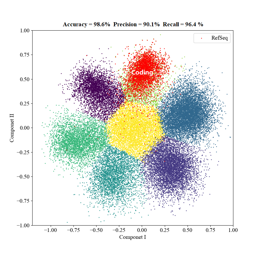
The picture below is the visualization of the self-training model obtained after 9-digit Z-curve transformation, principal component analysis and K-means clustering of all ORFs of Cupriavidus necator, which well explains why Z-curve is an effective method for gene identification.

6.1.2.6. ZcurveEncoder.dinucl_phase_transform

Do phasic dinucleotide transformation on a DNA sequence. Generate 36 parameters.

Definition
Let \(NA^i_n\), \(NG^i_n\), \(NC^i_n\), \(NT^i_n\) be the counts of dinucleotides in a DNA sequence of length \(n\) at position 1, 4, 7 …(i = 1), 2, 5, 8 …(i = 2) and 3, 6, 9 (i = 3), such that the phasic dinucleotide Z-curve transformation can be:

\(X^i_n = (NA^i_n + NG^i_n) - (NC^i_n + NT^i_n)\)
\(Y^i_n = (NA^i_n + NC^i_n) - (NG^i_n + NT^i_n),i=1,2,3\)
\(Z^i_n = (NA^i_n + NT^i_n) - (NC^i_n + NG^i_n)\)

It could also be defined using frequency of bases, which means a kind of normalized version, like:

\(x^i_n = [p^i_n({\rm NA}) + p^i_n({\rm NG})] - [p^i_n({\rm NC}) + p^i_n({\rm NT})]\)
\(y^i_n = [p^i_n({\rm NA}) + p^i_n({\rm NC})] - [p^i_n({\rm NG}) + p^i_n({\rm NT})],i=1,2,3\)
\(z^i_n = [p^i_n({\rm NA}) + p^i_n({\rm NA})] - [p^i_n({\rm NA}) + p^i_n({\rm NA})]\)

For more information, please see: ZcurvePy.ZcurveEncoder.k_nucl_phase_transform

Usage Example

from Bio import SeqIO
record = SeqIO.read("example.fa", "fasta")
encoder = ZcurveEncoder(record)
params = encoder.dinucl_phase_transform()
# params = encoder.dinucl_phase_transform(freq=True)

Application Scene
Gene recognition; Machine learning; Deep learning

Args:

• phase (int):
  the number of phases (default: 3)

• freq (bool):
  do frequencization or not (default: False)

• local (bool):
  use local mode to do frequencization

Returns:

• ndarray:
  Z-curve parameters

6.1.2.7. ZcurveEncoder.trinucl_phase_transform

Do phasic trinucleotide transformation on a DNA sequence. Generate 144 parameters.

Definition
Let \(XYA^i_n\), \(XYG^i_n\), \(XYC^i_n\), \(XYT^i_n\) be the counts of trinucleotides in a DNA sequence of length \(n\) at position 1, 4, 7 …(i = 1), 2, 5, 8 …(i = 2) and 3, 6, 9 (i = 3), such that the phasic trinucleotide Z-curve transformation can be:

\(X^i_n = (XYA^i_n + XYG^i_n) - (XYC^i_n + XYT^i_n)\)
\(Y^i_n = (XYA^i_n + XYC^i_n) - (XYG^i_n + XYT^i_n),i=1,2,3\)
\(Z^i_n = (XYA^i_n + XYT^i_n) - (XYC^i_n + XYG^i_n)\)

It could also be defined using frequency of bases, which means a kind of normalized version, like:

\(x^i_n = [p^i_n({\rm XYA}) + p^i_n({\rm XYG})] - [p^i_n({\rm XYC}) + p^i_n({\rm XYT})]\)
\(y^i_n = [p^i_n({\rm XYA}) + p^i_n({\rm XYC})] - [p^i_n({\rm XYG}) + p^i_n({\rm XYT})],i=1,2,3\)
\(z^i_n = [p^i_n({\rm XYA}) + p^i_n({\rm XYA})] - [p^i_n({\rm XYA}) + p^i_n({\rm XYA})]\)

For more information, please see: ZcurvePy.ZcurveEncoder.k_nucl_phase_transform

Usage Example

from Bio import SeqIO
record = SeqIO.read("example.fa", "fasta")
encoder = ZcurveEncoder(record)
params = encoder.trinucl_phase_transform()
# params = encoder.trinucl_phase_transform(freq=True)

Application Scene
Gene recognition; Machine learning; Deep learning

Args:

• phase (int):
  the number of phases (default: 3)

• freq (bool):
  do frequencization or not (default: False)

• local (bool):
  use local mode to do frequencization

Returns:

• ndarray:
  Z-curve parameters

6.1.2.8. ZcurveEncoder.k_nucl_phase_transform

Do phasic k-nucleotide transformation on a DNA sequence. Generate 9 x 4^(k-1) parameters.

Background
The Z-curve is an intuitive method for sequence visualization that can display purine versus pyrimidine, amino versus keto and strong H-bonded versus weak H-bonded bases along the DNA sequence. Sequence characteristics, including base composition distribution and periodicity patterns, are well displayed using the Z-curve method. Based on this method, numerous valuable tools for sequence analysis have been developed, contributing to our understanding of DNA sequences, and uncovering new biological insights. In general, the Z-curve method opens a new area of genome analysis using a geometric approach and provides an example of an innovative and systematic study.

Definition
Let \(N_{k-1}A^i_n\), \(N_{k-1}G^i_n\), \(N_{k-1}C^i_n\), \(N_{k-1}T^i_n\) be the counts of k-nucleotides in a DNA sequence of length \(n\) at position 1, 4, 7 …(i = 1), 2, 5, 8 …(i = 2) and 3, 6, 9 (i = 3), such that the phasic trinucleotide Z-curve transformation can be:

\(X^i_n = (N_{k-1}A^i_n + N_{k-1}G^i_n) - (N_{k-1}C^i_n + N_{k-1}T^i_n)\)
\(Y^i_n = (N_{k-1}A^i_n + N_{k-1}C^i_n) - (N_{k-1}G^i_n + N_{k-1}T^i_n),i=1,2,3\)
\(Z^i_n = (N_{k-1}A^i_n + N_{k-1}T^i_n) - (N_{k-1}C^i_n + N_{k-1}T^i_n)\)

It could also be defined using frequency of bases, which means a kind of normalized version, like:

\(x^i_n = [p^i_n({\rm N_{k-1}A}) + p^i_n({\rm N_{k-1}G})] - [p^i_n({\rm N_{k-1}C}) + p^i_n({\rm N_{k-1}T})]\)
\(y^i_n = [p^i_n({\rm N_{k-1}A}) + p^i_n({\rm N_{k-1}C})] - [p^i_n({\rm N_{k-1}G}) + p^i_n({\rm N_{k-1}T})],i=1,2,3\)
\(z^i_n = [p^i_n({\rm N_{k-1}A}) + p^i_n({\rm N_{k-1}T})] - [p^i_n({\rm N_{k-1}G}) + p^i_n({\rm N_{k-1}C})]\)

Usage Example

from Bio import SeqIO
record = SeqIO.read("example.fa", "fasta")
encoder = ZcurveEncoder(record)
params = encoder.k_nucl_phase_transform(k=2, phase=3, local=True)

Application Scene
Gene recognition; Machine learning; Deep learning

Args:

• k (int):
  the length of k-nucleotide (default: 3)

• phase (int):
  the number of phases (default: 3)

• freq (bool):
  do frequencization or not (default: False)

• local (bool):
  use local mode to do frequencization

Returns:

• ndarray:
  Z-curve parameters

6.1.2.9. ZcurveEncoder.genome_order_index

Calculate the genome order index of a nucleic sequence.

Background
Zhang CT and Zhang R has calculated the statistical quantity S for each of 809 genomes (11 archaea, 42 bacteria, 3 eukaryota, 90 phages, 36 viroids and 627 viruses) and 236 plasmids, found that S < 1/3 is strictly valid for almost all of the above genomes or plasmids. As a direct deduction of the above observation, it is shown that the statistical quantity S is a kind of genome order index, which is correlated with the Shannon function negatively. S < 1/3 suggests that a minimal value of the Shannon H function is required for each genome and should be anew biological statistical quantity useful to describe the composition features of genomes.

Definition
Let \(a\), \(g\), \(c\) and \(t\) be the frequency of A, G, C, T bases in a DNA sequence, such that the genome order index could be defined as:

\(S=a^2+g^2+c^2+t^2\)

Application Scene
Genome Analysis; Machine Learning

Usage Example

from Bio import SeqIO
record = SeqIO.read("example.fa", "fasta")
encoder = ZcurveEncoder(record)
value = encoder.genome_order_index()

Returns:

• float:
  Genome order index

6.1.2.10. ZcurveEncoder.RY_order_index

Calculate the RY order index of a nucleic sequence

Definition
Let \(a\), \(g\), \(c\) and \(t\) be the frequency of A, G, C, T bases in a DNA sequence, such that the RY order index could be defined as:

\(S=(a+g)^2+(c+t)^2\)

Application Scene
Genome Analysis; Machine Learning

Usage Example

from Bio import SeqIO
record = SeqIO.read("example.fa", "fasta")
encoder = ZcurveEncoder(record)
value = encoder.RY_order_index()

Returns:

• float:
  RY order index

6.1.2.11. ZcurveEncoder.MK_order_index

Calculate the MK order index of a nucleic sequence

Definition
Let \(a\), \(g\), \(c\) and \(t\) be the frequency of A, G, C, T bases in a DNA sequence, such that the MK order index could be defined as:

\(S=(a+c)^2+(g+t)^2\)

Application Scene
Genome Analysis; Machine Learning

Usage Example

from Bio import SeqIO
record = SeqIO.read("example.fa", "fasta")
encoder = ZcurveEncoder(record)
value = encoder.MK_order_index()

Returns:

• float:
  MK order index

6.1.2.12. ZcurveEncoder.WS_order_index

Calculate the WS order index of a nucleic sequence

Definition
Let \(a\), \(g\), \(c\) and \(t\) be the frequency of A, G, C, T bases in a DNA sequence, such that the WS order index could be defined as:

\(S=(a+t)^2+(g+c)^2\)

Application Scene
Genome Analysis; Machine Learning

Usage Example

from Bio import SeqIO
record = SeqIO.read("example.fa", "fasta")
encoder = ZcurveEncoder(record)
value = encoder.WS_order_index()

Returns:

• float:
  WS order index

6.1.2.13. ZcurveEncoder.AT_order_index

Calculate the AT order index of a nucleic sequence

Definition
Let \(a\) and \(t\) be the frequency of A and T bases in a DNA sequence, such that the AT order index could be defined as:

\(S=a^2+t^2\)

Application Scene
Genome Analysis; Machine Learning

Usage Example

from Bio import SeqIO
record = SeqIO.read("example.fa", "fasta")
encoder = ZcurveEncoder(record)
value = encoder.AT_order_index()

Returns:

• float:
  AT order index

6.1.2.14. ZcurveEncoder.GC_order_index

Calculate the GC order index of a nucleic sequence

Definition
Let \(g\) and \(c\) be the frequency of G and C bases in a DNA sequence, such that the GC order index could be defined as:

\(S=g^2+c^2\)

Application Scene
Genome Analysis; Machine Learning

Usage Example

from Bio import SeqIO
record = SeqIO.read("example.fa", "fasta")
encoder = ZcurveEncoder(record)
value = encoder.GC_order_index()

Returns:

• float:
  GC order index

6.1.3. BatchZcurvePlotter

A multithreaded version of ZcurvePlotter for processing dataset using Z-curve as embedding method in deep learning. Note that this API’s functional richness is far less than the latter.

Usage Example:

from Bio import SeqIO

records = SeqIO.parse("sequences.fa", "fasta")
plotter = BatchZcurvePlotter(mode='accum', n_jobs=8)
z_values = plotter(records)

plotter = BatchZcurvePlotter(mode='profile', n_jobs=8)
z_values, k_values = plotter()

Args:

• mode (str):
  The mode to processing sequences:
  (1) ‘accum’ means cumlulative curves;
  (2) ‘profile’ means fitted curves;
  (3) ‘tetra’ means no accumulations.

• window (int):
  window size used by mean-smoothing method. If a value <= 0 is given, do nothing and return the original curve data.(Default:0)

• n_jobs (int):
  specifies the number of threads to use. If it is set to a negative value or 0, it will be reset to the number of CPU cores of the machine. (Default: -1)

Returns:

• object: _ZcurvePy.BatchZcurvePlotter

6.1.4. BatchZcurveEncoder

The multi-thread version of ZcurveEncoder with simpler syntax. More suitable for extracting features on large datasets.

Usage Example

from ZcurvePy import BatchZcurveEncoder
# Define the hyper-paramsfor 765-bit Z-curve transform
hyper_params = [
    {"k": 1, "freq": True}  # Same as mononucl_phase_transform(freq=True)
    {"k": 2, "freq": True}  # Same as dinucl_phase_transform(freq=True)
    {"k": 3, "freq": True}  # Same as trinucl_phase_transform(freq=True)
    {"k": 4, "freq": True}  # Same as k_nucl_phase_transform(k=4, freq=True)
]
encoder = BatchZcurveEncoder(hyper_params, n_jobs=8)
features = encoder(records)

Args:

• hyper_params (list):
  JSON styled object that defines the hyper-parameters for Z-curve transformation. For example, the following content tells the BatchZcurveEncoder to do a mononucleotide non-phase Z-curve t.f. and a trinucleotide phase-specific Z-curve t.f. to every item, then concatenate them as a 147-dim feature vector:

  [{'k': 1, 'phase': 1, 'local': True}, {'k': 3, 'phase': 3, 'local': True}]
  

  For the meaning of the variable names, see the APIs of ZcurvePy.ZcurveEncoder.

  • k (int):
    must be given >= 1, and preferably not more than 6. (Default: None)

  • phase (int):
    must be given >= 1, and preferably not more than 6. (Default: 3)

  • freq (bool): when ‘local’ is true, freq is forced to be true. (Default: False)

  • local (bool): note that for k and phase=1, the local mode yields the same values as when only freq is set to be true. (Default: False)

• n_jobs (int):
  specifies the number of threads to use. If it is set to a negative value or 0, it will be reset to the number of CPU cores of the machine. (Default: -1)

Returns:

• object: _ZcurvePy.BatchZcurveEncoder

6.1.5. ZcurveSegmenter

Z-curve segmenter based on genome order number, which can be considered an extended version of the GC-Profile’s core. It has 7 modes and can be used for edge recognition of genomic islands, CpG islands, AT-rich regions and other structures.

6.1.5.1. ZcurveSegmenter.__init__

The __init__ function of ZcurvePy.ZcurveSegmenter.

Args:

• mode (str):
  The mode Z-curve segmenter. It can be one of the following:

  • ‘GN’: Using genome order number to segment Z-curves;

  • ‘RY’: Using RY order number to segment RY-profile;

  • ‘MK’: Using MK order number to segment MK-profile;

  • ‘WS’: Using WS order number to segment GC-profile;

  • ‘AT’: Using AT order number to segment AT-skew;

  • ‘GC’: Using GC order number to segment GC-skew;

  • ‘CG’: Using CpG order number to segment CpG-profile.

• halting (int):
  The halting value of segmenter. Defaults to 100.

• min_len (int):
  The minimum length of fragments. Defaults to 3000.

• max_depth (int):
  The maximum depth of iteration. Defaults to 9999.

6.1.5.2. ZcurveSegmenter.run

Run the segmenter.

Args:

• record (str):
  The sequence to be segmented.

Returns:

• list:
  A list of tuples, each tuple contains the position and the value of the segment point.

6.1.5.3. ZcurveSegmenter.reset

Reset the segmenter. Clear segmentation points generated in the last run.

6.1.6. ZcurveBuilder

A simple API for building gene recognizer. It includes basic modules such as feature extraction, preprocessing, negative sampling and model training. Each module is customizable. Core algorithm of ZCURVE 2.0 / 3.0.

Usage Example

from ZcurvePy.RunnableScriptsUtil import download_acc, extract_CDS
from ZcurvePy import ZcurveBuilder
from Bio.SeqIO import read, parse
# Load positive dataset
path = download_acc("NC_000913.3")[0]
pos_dataset = extract_CDS(path)
builder = ZcurveBuilder(standard=True, n_jobs=8)
builder.fit(pos_dataset)
# Some sample sequences
records = parse("samples.fa", "fasta")
results = builder.predict(records)

6.1.6.1. ZcurveBuilder.__init__

The __init__ function of ZcurvePy.ZcurveBuilder

Args:

• encoder (Callable):
  A function or object that can be called with a list of supported sequences and returns a feature matrix of the data set. Default is a BatchZcurveEncoder object that yields 189-dim features.

• model (object):
  A machine learning model object that have fit and predict_proba method. Default is a RBF-SVM model from sklearn.svm.SVC with balanced class weights.

• standard (bool):
  Whether to apply standardization to the data. (Use sklearn.preprocessing.StandardScaler)
  Default: True

• normal (bool):
  Whether to apply normalization to the data. (Use sklearn.preprocessing.MinMaxScaler)
  Default: False

• neg_pos_ratio (int):
  The ratio between negative samples and positive samples, decides how many negative sequences should be obtained from each positive case sequence.
  Parameter for ZcurveBuilder.shuffle, default is 5.

• seed (int):
  Random seed.

• n_jobs (int):
  Number of CPU cores used. All are used by default.

Returns:

• object: ZcurvePy.ZcurveBuilder

6.1.6.2. ZcurveBuilder.fit

Fit the model after negative samples are generated and the dataset is preprocessed.

Args:

• pos_data (object):
  Positive example sequence data sets generally use reference gene sequences as positive examples.

6.1.6.3. ZcurveBuilder.predict

Predict whether a set of sequences is a gene coding sequence.

Args:

• data (object):
  Sequence dataset to predict.

• threshold (float):
  Label judgment threshold.
  Greater than the threshold is a positive sample, and less than the threshold is a negative sample.

Returns:

• labels (ndarray):
  Prediction label for the sample.

• scores (ndarray):
  The predicted score of the sample.

6.1.7. decode

ZcurvePy.decode(*args, **kwargs)

Decode Z-curves to DNA sequences. Only the three 3D curves provided by BatchZcurvePlotter can be reduced to DNA sequences, so this API is actually the reverse of the latter. Multi-thread is supported.

Usage Example:

from Bio import SeqIO
from ZcurvePy import BatchZcurvePlotter, decode

records = SeqIO.parse("sequences.fa", "fasta")
plotter = BatchZcurvePlotter(mode='accum', n_jobs=8)
z_values = plotter(records)
sequences = decode(z_values)

Args:

• data (list):
  Data of curves to be decode.

• k_values (list):
  Auxiliary slope information used to decode the fitted curves \((x', y', z')\).

• mode (str): the mode to processing sequences:
  ‘accum’ means cumlulative curves; ‘profile’ means fitted curves; ‘tetra’ means no accumulations.

• n_jobs (int):
  Specifies the number of threads to use. If it is set to a negative value or 0, it will be reset to the number of CPU cores of the machine. (Default: -1)

Returns:

• seqs (list): list of sequences as str.

6.1.8. shuffle

ZcurvePy.shuffle(*args, **kwargs)

Do Fisher-Yates shuffle to the bases in a sequence. This API’s operands are batch datasets and supports multi-threads.

Background
In the development of ZCURVE system, it is a rather difficult problem to prepare an appropriate set of non-coding sequences in bacterial genomes, because the amount of non-coding DNA is too few to be used. To solve this problem, the shuffle method to produce negative samples is presented.

Application Scene
Gene recognition; Machine Learning

Usage Example

from Bio import SeqIO
records = SeqIO.parse('examples.fa', 'fasta')
shufseq = shuffle(records)

Args:

• records (list):
  Sequence dataset to be processed, str, Bio.Seq.Seq, Bio.SeqRecord.SeqRecord and many types are supported.

• ratio (int):
  The ratio between negative samples and positive samples, decides how many negative sequences should be obtained from each positive case sequence.

• seed (int):
  Random seed.

• n_jobs (int):
  Specifies the number of threads to use. If it is set to a negative value or 0, it will be reset to the number of CPU cores of the machine. (Default: -1)

Returns:

• shufseqs (list):
  Shuffled sample sequences.

6.2. Third-party API

We list all of the third party APIs we call here.

API	Description	Python Package
numpy.array	Convert objects to numpy.ndarray.	Numpy
Bio.Seq	Provide objects to represent biological sequences with alphabets.	Biopython
Bio.SeqRecord	Represent a Sequence Record, a sequence with annotation.	Biopython
Bio.SeqIO	The standard Sequence Input/Output interface.	Biopython
Bio.SeqUtils	Miscellaneous functions for dealing with sequences.	Biopython
matplotlib.pyplot	State-based interface to matplotlib.	Matplotlib
sklearn.preprocess	Data preprocessing module including standardization and normalization.	Sci-kit Learn
sklearn.svm	Support vector machine models.	Sci-kit Learn